
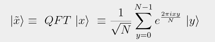
The mathematical foundation behind Grover’s diffusion operator — derived from first principles.
In the Grover’s Algorithm — Inversion About the Mean walkthrough, the diffusion operator applies H⊗³ twice per iteration. Every single step is governed by a sign table called the Hadamard Reference. That table is not a lookup shortcut — it is the 8×8 Walsh-Hadamard Transform matrix written out in full. This post derives it from scratch: one qubit, then two, then all three, arriving at the complete matrix and the rule behind every sign in it.
We initialise all three qubits in the ground state |0⟩ and route each through its own independent Hadamard gate. There are no two-qubit (entangling) gates here — the circuit is entirely parallel.
| Qubit | Input | Gate | Output ket |
|---|---|---|---|
| q₀ | |0⟩ | H | (1/√2)( |0⟩ + |1⟩ ) |
| q₁ | |0⟩ | H | (1/√2)( |0⟩ + |1⟩ ) |
| q₂ | |0⟩ | H | (1/√2)( |0⟩ + |1⟩ ) |
All three outputs are identical because all three inputs are identical. The structure we need emerges when we take their tensor product.
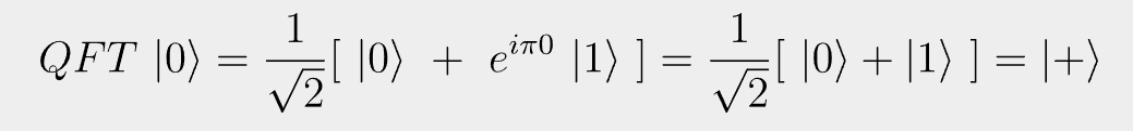
The Hadamard gate H maps the two computational basis states as follows:
| Input | H |input⟩ | Short notation |
|---|---|---|
| |0⟩ | (1/√2)( |0⟩ + |1⟩ ) | |+⟩ |
| |1⟩ | (1/√2)( |0⟩ − |1⟩ ) | |−⟩ |
In matrix form:
+1 −1
Expanding the tensor product of the first two post-H qubits:
= (1/√2)(|0⟩ + |1⟩) ⊗ (1/√2)(|0⟩ + |1⟩)
= (1/2)( |0⟩⊗|0⟩ + |0⟩⊗|1⟩ + |1⟩⊗|0⟩ + |1⟩⊗|1⟩ )
= (1/2)( |00⟩ + |01⟩ + |10⟩ + |11⟩ )
Adding the third qubit expands the superposition to all 8 three-bit strings:
= (1/√2)³ (|0⟩+|1⟩) ⊗ (|0⟩+|1⟩) ⊗ (|0⟩+|1⟩)
= (1/√8)( |000⟩ + |001⟩ + |010⟩ + |011⟩
+ |100⟩ + |101⟩ + |110⟩ + |111⟩ )
When H⊗³ is applied to an arbitrary basis state |j⟩, the result is:
The entry at row i, column j carries sign (−1)popcount(i AND j) divided by √8. The table below shows all 64 signs — green (+) for +1/√8 and red (−) for −1/√8:
| H⊗³ |j⟩ → output |i⟩ ↓ |
|000⟩ | |001⟩ | |010⟩ | |011⟩ | |100⟩ | |101⟩ | |110⟩ | |111⟩ |
|---|---|---|---|---|---|---|---|---|
| H|000⟩ | + | + | + | + | + | + | + | + |
| H|001⟩ | + | − | + | − | + | − | + | − |
| H|010⟩ | + | + | − | − | + | + | − | − |
| H|011⟩ | + | − | − | + | + | − | − | + |
| H|100⟩ | + | + | + | + | − | − | − | − |
| H|101⟩ | + | − | + | − | − | + | − | + |
| H|110⟩ | + | + | − | − | − | − | + | + |
| H|111⟩ | + | − | − | + | − | + | + | − |
Because H acts independently on each qubit, H⊗³ is the tensor product of three 2×2 matrices. The entry at row i, column j is simply the product of the three corresponding single-qubit entries:
Each single-qubit factor equals +1 unless both the k-th bit of i and the k-th bit of j are 1, in which case it equals −1. So the k-th factor contributes a sign of (−1)iₖ·jₖ. Multiplying all three:
Quick verification: row H|101⟩, column |011⟩
| i (row) | j (col) | i AND j | popcount | Sign |
|---|---|---|---|---|
| 101 (= 5) | 011 (= 3) | 001 | 1 (odd) | − ✓ |
Matches the matrix in Section 5: row H|101⟩, column |011⟩ is indeed −.
This matrix is the Hadamard Reference table used throughout the Grover’s Algorithm — Inversion About the Mean post. The diffusion operator D = H⊗³ (2|0⟩⟨0| − I) H⊗³ works in three sub-steps, each directly using this matrix:
| Sub-step | Operation | Grover walkthrough steps |
|---|---|---|
| First H⊗³ | Maps computational basis → Hadamard basis. Each amplitude spreads across all 8 columns via the sign table. | 4.1 · 6.1 · 8.1 |
| Phase flip | 2|0⟩⟨0|−I: keeps |000⟩ unchanged, negates all other states. This is the inversion-about-the-mean mechanism. | 4.2 · 6.2 · 8.2 |
| Second H⊗³ | Maps back to computational basis using the same sign table (H is self-inverse). Routes constructive interference into the target state. | 4.3 · 6.3 · 8.3 |
Quantum Series 2026 · Built with Qiskit 1.x
✦ This article was generated with the assistance of Claude by Anthropic ✦

You must be logged in to post a comment.